15.1 Use Case 1: Represent an Optical Fiber Installation

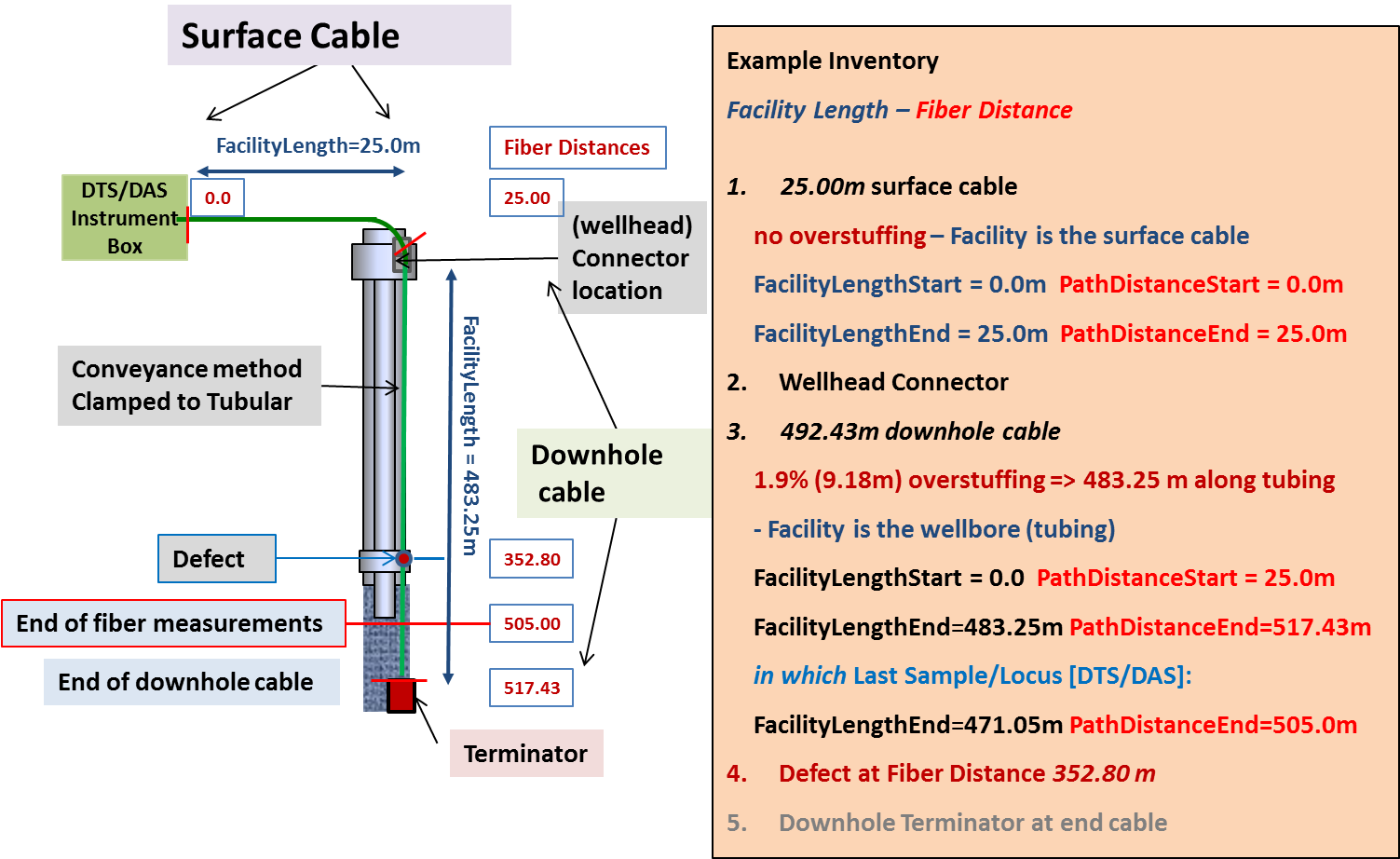
This section contains examples of XML code for representing a typical common style of fiber installation (Figure 15.1-1). There are two fiber segments of 25m and 492.43m, giving a total distance of 517.43m. There is overstuffing of 1.9% in the downhole fiber segment, giving it a length along the facility of 483.25m. Two facility mappings are made: 1) the surface cable, which is one to one, and 2) the downhole cable mapped to the wellbore, which includes the effects of the offset to the wellhead and of the overstuffing.

Figure 15.1-1 Worked example fiber optical path showing fiber segments, optical path lengths and facility lengths

For the optical path shown in Figure 15.1-1 , the key sections are as shown below.

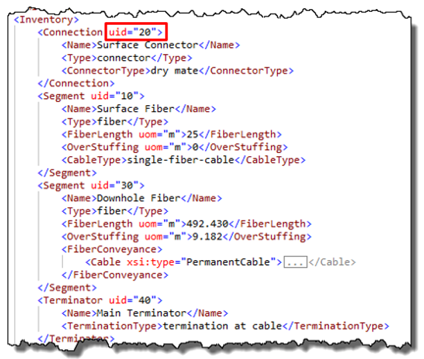
First, the inventory lists out the components comprising the optical path (Figure 15.1-2). Note that each component has a name and a type (and optionally additional data), and also a uid (red box) which is used to reference this component from the network (see below).

Figure 15.1-2 Inventory section of the Optical Path.

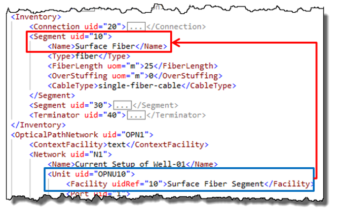
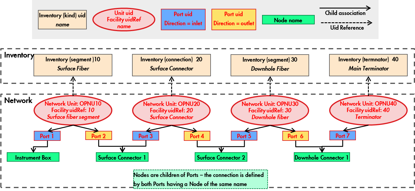
Next, the Network section shows how these components listed in Inventory are connected. (For details on how this is done, see 14.3.3 Optical Path Network Representation , Figure 14.3.3-1 .) The network contains Units which are a nominal representation of an item of inventory ("facility" is the Energistics terminology for general hardware) within the network. Figure 15.1-3 shows a network Unit (blue box), which uses a facility reference (uidRef) back to the uid of the component in Inventory (red box).

Figure 15.1-3 Network section of Optical Path showing reference to Inventory.

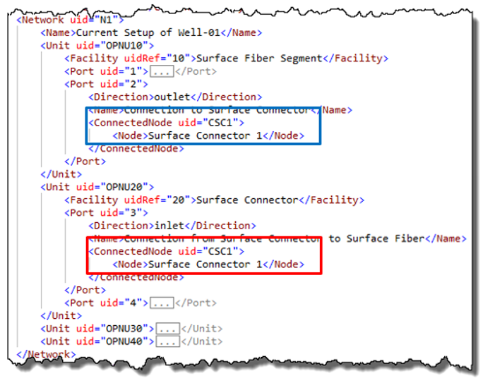
The unit has one or more Ports which are where connection occurs. Ports can be inlet or outlet (taking direction from the lightbox). Ports contain a Connected Node element, and where two ports share the same name and uid of Node, this defines their connection. See Figure 15.1-4 , in which the outlet port (i.e., “far end”) of the surface fiber (in blue box), can be seen to be connected to the inlet port (i.e., “near end”) of the surface connector (in red box). Both have a connected node called Surface Connector 1 with uid CSC1, which defines the connection between the surface cable and this wellhead connector.

Figure 15.1-4 Optical path network showing Node connecting Ports of two components.

In Figure 15.1-5 , we see the full inventory and network of the worked example with the links and connections all shown.

Figure 15.1-5 Worked example optical path network showing how connectivity is defined.

The facility mapping section is where the fiber optical path distances are mapped onto the facility lengths of physical equipment. Here, two mappings are shown: 1) a one-to-one mapping to the surface cable from the surface segment of the optical path and 2) a mapping to the wellbore, which includes the offset and the overstuffing, as shown in Figure 15.1-1 . Figure 15.1-6 shows the two mappings. Note that the FiberFacilityWell type of mapping (the second one) includes a well datum and a data object reference to the wellbore concerned.

Figure 15.1-6 Facility Mapping section of the Optical Path.

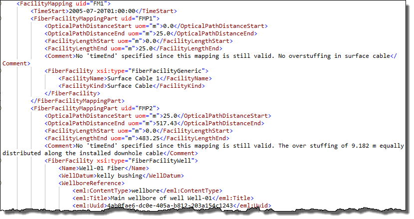
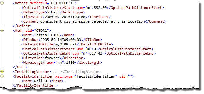
Figure 15.1-7 shows some of the other sections of the Optical Path. Defects can be recorded (for the example, see Figure 15.1-1 and, for real-world defect examples, see Figure 14.3.5-1 ). OTDR surveys to verify the optical path quality can be referenced. The data for OTDR are not in an Energistics standard because OTDR is a generic fiber optical industry measurement with its own file formats; an external file is referenced. Other data can be added as seen, such as vendor, the facility identifier, etc.

Figure 15.1-7 Defect, OTDR, and other sections of Optical Path.