11.19.7 Higher Order Finite Element Prism24 Unstructured Column-layer Grid

This example demonstrates an unstructured column-layer grid representation and the use of higher order subnode geometry to create a distorted prism cell shape. For simplicity, this example is of an unfaulted grid.

Figure 11.19.7-1 Description of a single lower order (blue prism) and higher (distorted prism) grid cell. All nine edges are distorted but not all are shown.

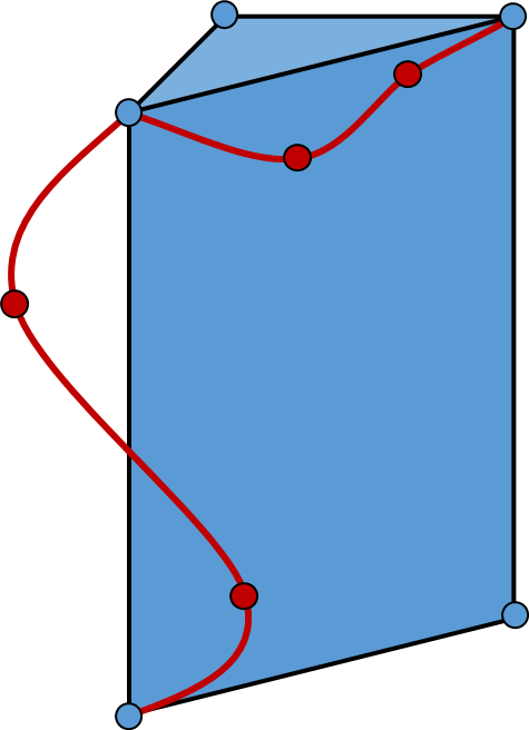
As shown in Figure 11.19.7-1 , there are six blue nodes, defining the shape of the lower order triangular prism. There are two additional higher order nodes per edge, for each of the nine edges, which describe the distortion of each edge away from linearity. (Only two edges are shown.) The resulting distorted prism is described by a total of 24 nodes.

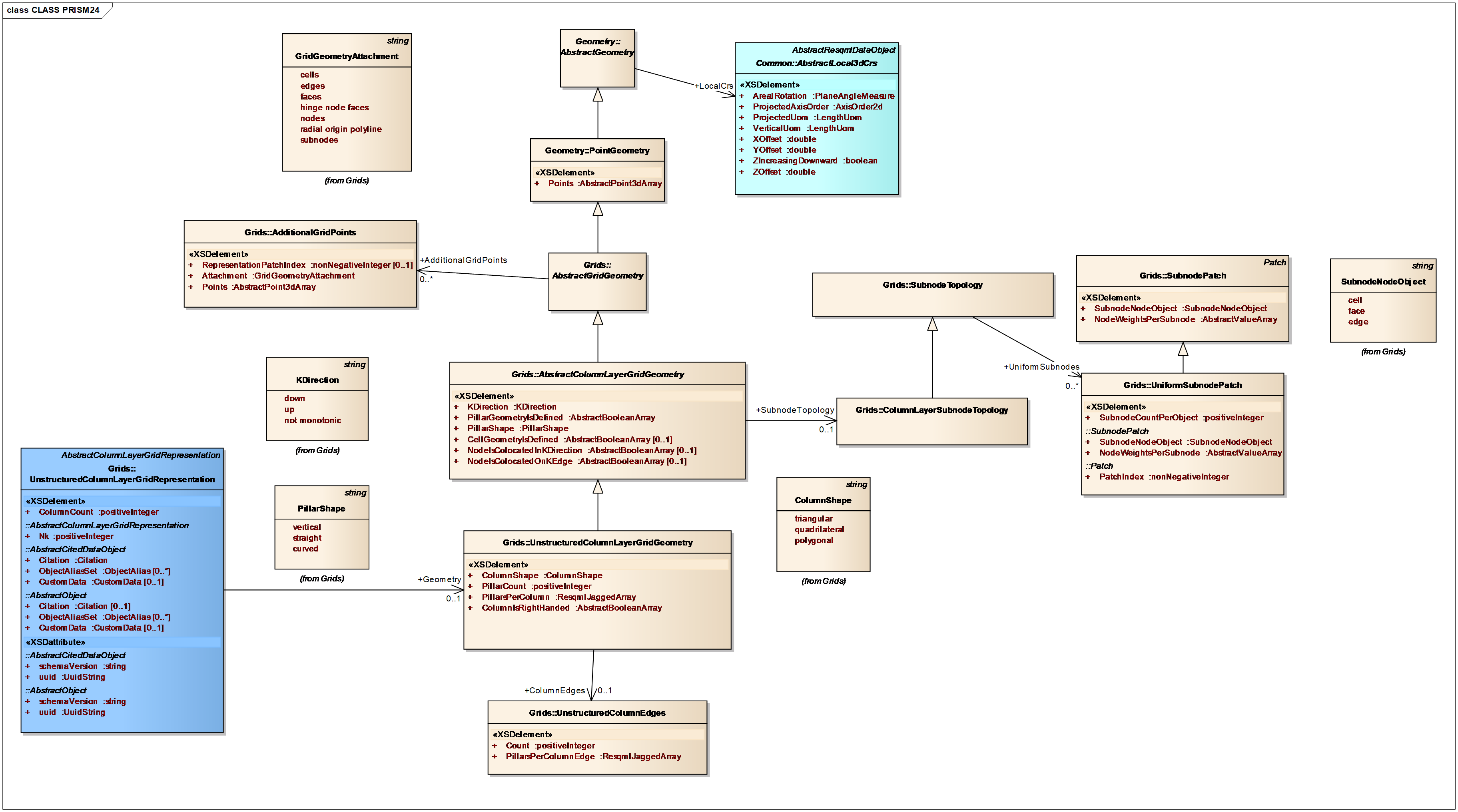
The description of the lower order aspects grid is similar to that of the IJK grid except that the grid uses an unstructured column-layer cell geometry (Figure 11.19.7-2). The unstructured column-layer cell geometry inherits from the column-layer cell geometry used for the IJK grid, but includes additional elements that explicitly describe the pillars and columns of the model. The higher order finite element grid is a simple kind, with two subnodes defined for each edge. The edges and the nodes per edge must be defined explicitly before they can be referenced by the subnode construction.

Figure 11.19.7-2 Class diagram for the Prism24 grid.

Figure 11.19.7-3 Instance diagram for the Prism24 grid.

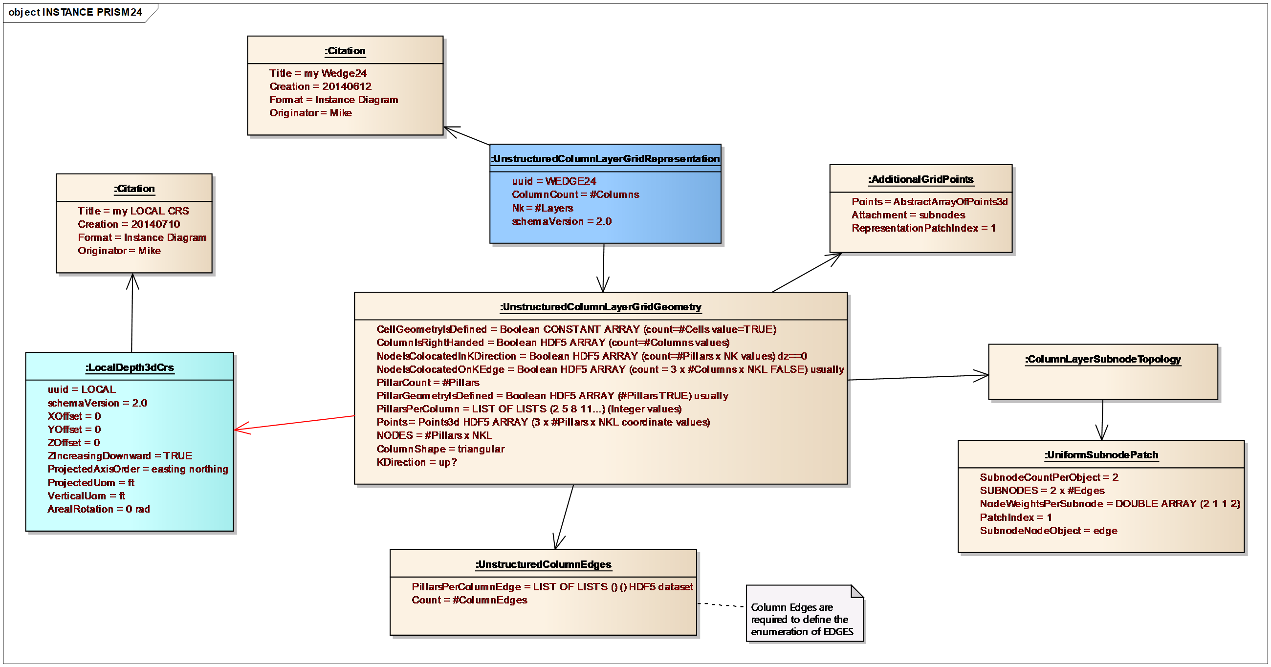
Section 11.13.3 Unstructured Column-Layer Grid Indexable Elements explains the edge indexing for an unstructured column-layer grid is given by “ColumnEdgeCount x NKL + CoordinateLineCount x NK + SplitEdgeCount”. In Figure 11.19.7-3 , the column edges are defined explicitly using a jagged array construction. Because the grid is unfaulted, the coordinate line count is identical to the pillar count. This model has no split edges, hence the edge indexing is known. There are two subnodes per edge, defined using the uniform subnode patch. Each subnode is defined parametrically by the two nodes per edge: the first with weights of (2 1) and the second with weights of (1 2). In other words, subnode1 = (2/3)*edgenode1 + (1/3)*edgenode2 while subnode2 = (1/3)*edgenode1 + (2/3)*edgenode2. Once defined, these subnodes may be used to provide topological support for higher order properties or geometry. In this example, the positions of the subnodes are modified when higher order geometry points are attached, giving the distorted shape. As a reminder, the schema itself does not describe the method of geometric interpolation between the subnodes on an edge or between the subnodes on a face, although natural interpolation algorithms do arise. For instance, in this figure, edge interpolation follows a natural cubic spline and face interpolation follows the iso-parametric mapping of the lowest order object.