18.1.4 DAS Equipment and Data Types: Raw and Processed Data
| Topic Version | 1 | Published | 12/09/2016 | |
| For Standard | PRODML v2.0 | |||
Figure 18.1.4-1 shows basic DAS equipment configuration and usage and introduces some important concepts about the raw data and how it’s represented in the DAS PRODML data schemas, which are explained in Chapter 19 DAS: Data Model .
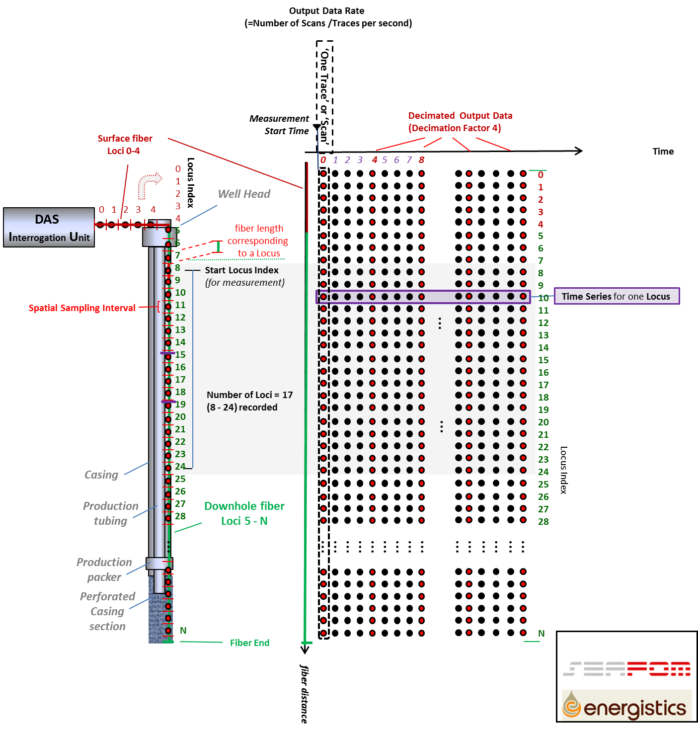
The DAS instrument box (or interrogation unit or IU) is connected to a sensing fiber. The sensing fiber consists of a surface part (surface fiber in the figure) and a downhole part (downhole fiber in the figure) together presenting the full fiber optical path. The DAS IU sends light pulses in the fiber at a pre-configured rate (interrogation or pulse rate), and samples the backscattered light creating an ensemble of N loci samples along the fiber. Such an ensemble is often referred to as a “trace” or “scan,” and is shown as columns of dots in the figure. The time at which a trace is collected is indicated by the measurement start time. A DAS IU interrogating the full fiber outputs a maximum of N x pulse rate “raw” DAS samples per second. Each locus sample is shown as a dot in Figure 18.1.4-1 .
In many cases the DAS IU is configured such that it decimates the output by an integer factor M and only outputs every M th trace. The rate at which scans are output by the interrogator is called the “output data rate.” The red dots in Figure 18.1.4-1 show such a decimation example (decimation factor 4).
Further, the DAS IUs often collect only measurements for a subset of the loci along the fiber. In Figure 18.1.4-1 , the shaded grey box indicates such a scenario where only loci 8 to 24 are collected. In the figure, “start locus index” and “number of loci” describe which subset is collected. To ensure a unique numbering system, the first locus at the interrogator has by definition index ‘0’.
Measurement samples output for a single locus can form a time series of samples, represented by rows of dots in the figure.
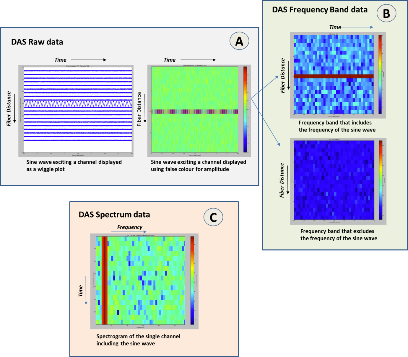
Figure 18.1.4-2 introduces a number of additional concepts when processing raw data into frequency bands and spectra using Fourier transforms. An example of the raw data is shown in box ‘A’ containing a representation of a sine wave exciting a single channel (locus) along the fiber (left plot) and the corresponding 'waterfall' DAS raw data plot (right plot in box A). When we now apply filters to this raw data, one filter which includes and one that excludes the sine wave’s frequency, then we obtain two processed filtered images shown in box ‘B’ referred two as processed DAS Frequency Band Extracted (FBE) data. We can also calculate the full signal frequency spectrum for each DAS channel using a Fast Fourier Transform shown in box ‘C which is referred to as Spectrum data.