7.3.1 Cubic Splines

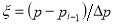
There are many ways to describe a cubic spline. The current description draws heavily upon the description in Numerical Recipes (Press et al. 1992), but with some variations that are in use within our domain. For a spline, each interval is parameterized in terms of a parameter p, or equivalently a normalized parameter , , . The parameter takes on the values of =0 and at the two knots that bound the interval. We may express a cubic spline in terms of its function values and second derivatives, specified at the two knots. 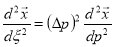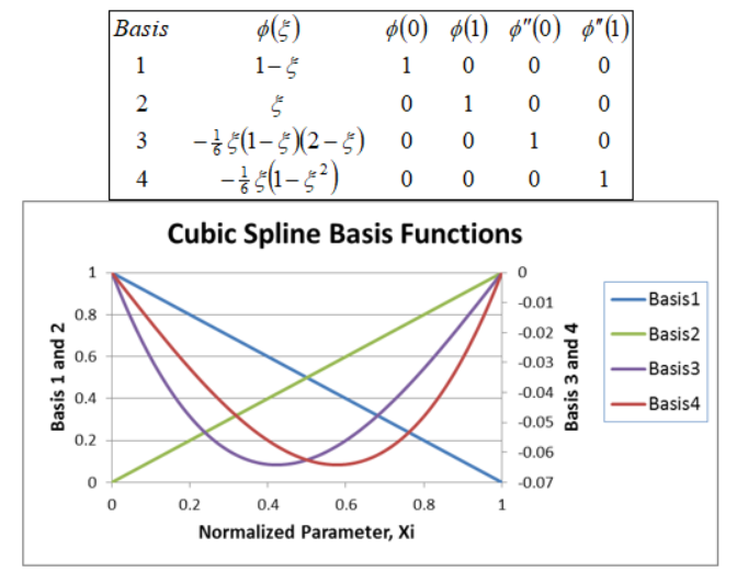Spline derivatives are specified with respect to the parameter p, but need to be converted to a derivative with respect to  within an interval, and , when using the following table of basis functions. Although the derivatives with respect to the parameter p may be continuous at the knots, because of the scaling by Δp, the normalized derivatives with respect toneed not be. The interpolant for a cubic spline can then be written as a superposition of four basis functions (Figure 7.3.1-1 ).

Figure 7.3.1-1 Cubic Spline Basis Functions.

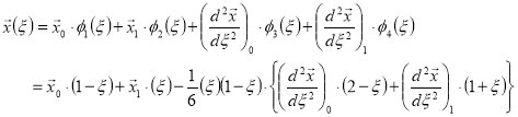
Specifically, within an interval we have:

For instance, a function that takes on the values of a and b at the interval knots but with vanishing second derivatives would be given by . With non-zero second derivatives, a cubic equation would arise. Any cubic spline may be expressed in this fashion, and all cubic splines rely upon the specification of the control points at the knots. However, different cubic spline implementations arise depending upon the specification of the derivatives at the knots.